Diagnostic classification models

A brief introduction

W. Jake Thompson, Ph.D.

What are diagnostic models?

• Traditional assessments and psychometric models measure an overall skill or ability
• Assume a continuous latent trait

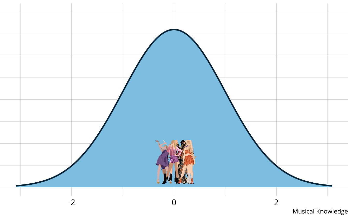
• The output is a weak ordering due to error in estimates
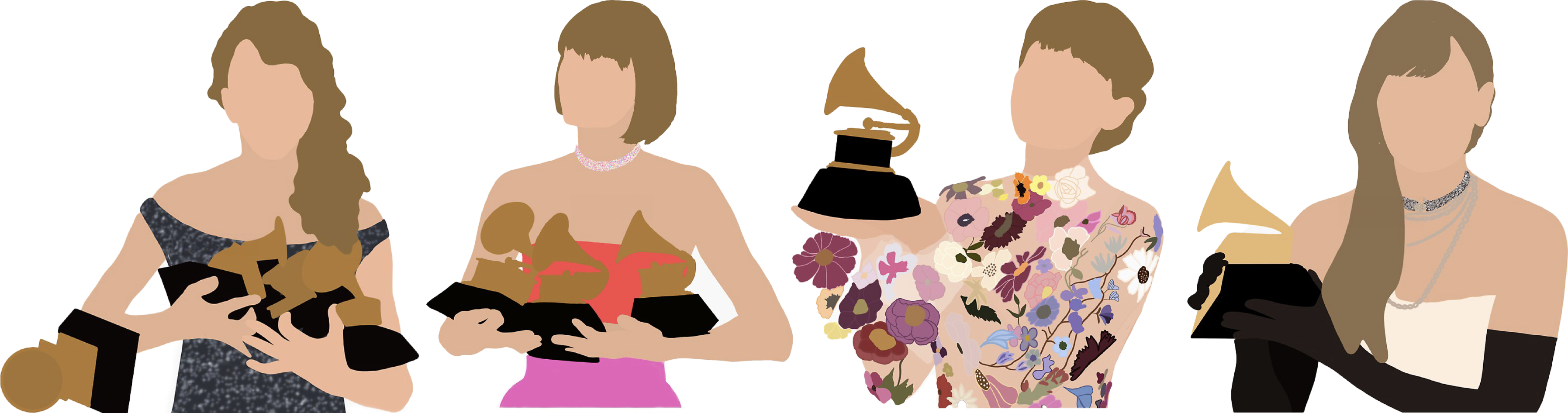
  • Confident Taylor Swift (debut) is the worst
  • Not confident on ordering toward the middle of the distribution

• Limited in the types of questions that can be answered.
  • Why is Taylor Swift (debut) so low?
  • What aspects do each era demonstrate proficiency or competency of?
  • How much skill is “enough” to be competent?

Diagnostic measurement

• Designed to be multidimensional
• No continuum of student achievement
• Categorical constructs
  • Usually binary (e.g., master/nonmaster, proficient/not proficient)
• Several different names in the literature
  • Diagnostic classification models (DCMs)
  • Cognitive diagnostic models (CDMs)
  • Skills assessment models
  • Latent response models
  • Restricted latent class models

Diagnostic music assessment

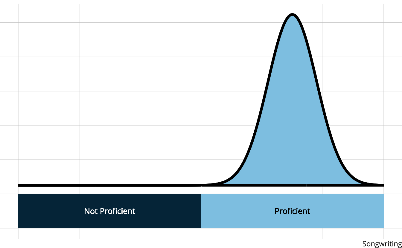
• Rather than measuring overall musical knowledge, we can break music down into set of skills or attributes
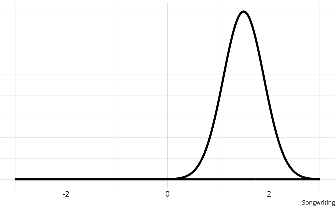
  • Songwriting
  • Production
  • Vocals

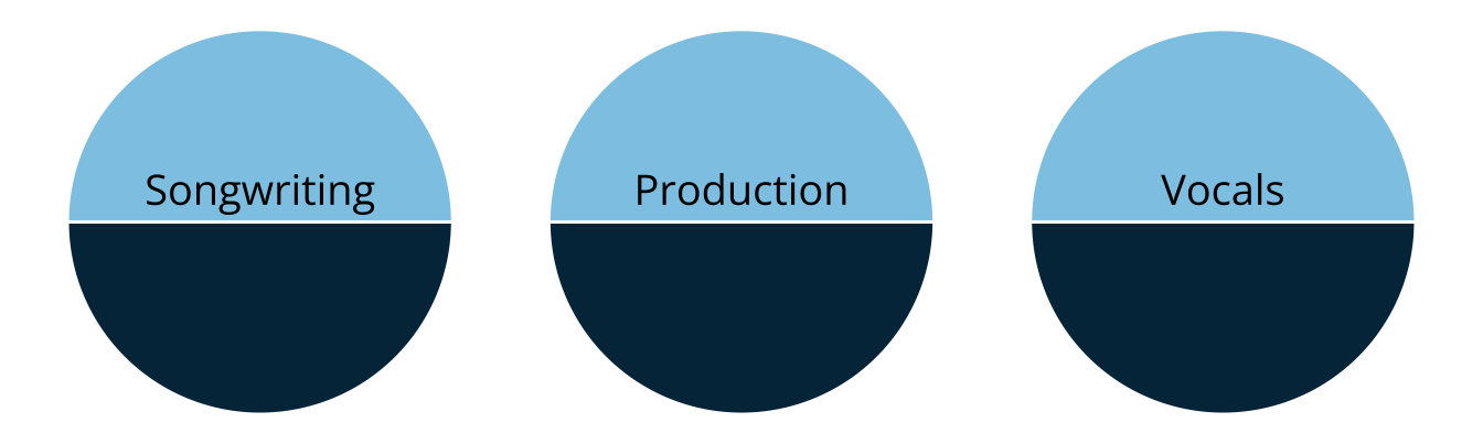
• Attributes are categorical, often dichotomous (e.g., proficient vs. non-proficient)

Diagnostic classification models

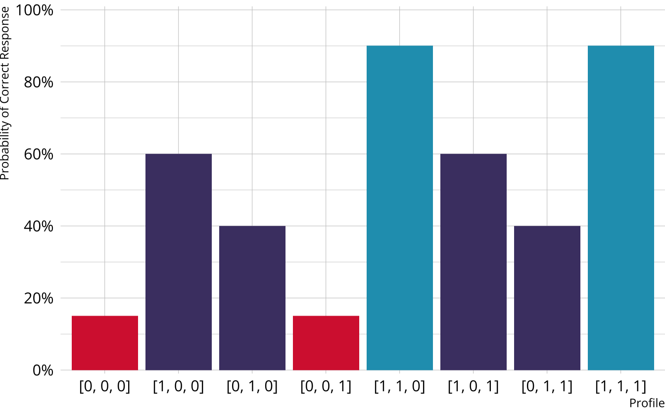
• DCMs place individuals into groups according to proficiency of multiple attributes

	songwriting	production	vocals

Benefits of DCMs

• Fine-grained, multidimensional results. Answer more questions:
  • Why is Taylor Swift (debut) so low?
    • Subpar songwriting, production, and vocals
  • What aspects are albums competent/proficient in?
    • DCMs provide classifications directly
• High reliability with fewer items
  • Less information need to classify than to place precisely along a scale

	songwriting	production	vocals

Results from DCM-based assessments

	songwriting	production	vocals

• No scale, no overall “ability”
• Students are probabilistically placed into classes
  • Classes are represented by skill profiles
• Feedback on specific skills as defined by the cognitive theory and test design

Fine-grained feedback

• Distinguish between respondents who may have similar scale scores

	songwriting	production	vocals

Item structures for DCMs

• Item structure: Which skills are measured by each item?

  • Simple structure: Item measures a single skill
  • Complex structure: Item measures 2+ skills

• Defined by Q-matrix

• Interactions between attributes when an item measures multiple skills driven by cognitive theory and/or empirical evidence

  • Can proficiency of one skill compensate for non-proficiency of another?
  • Are skill acquired in a particular order (e.g., hierarchy)?

item	songwriting	production	vocals
1	1	0	0
2	0	0	1
3	0	1	0
4	1	1	0
5	1	0	1
6	0	1	0
7	0	1	0
8	1	0	1
9	0	0	1
10	1	0	1
11	1	1	0
12	0	1	1
13	0	0	1
14	1	0	1
15	1	1	0
16	0	1	0
17	1	0	0
18	1	1	0
19	1	0	0
20	1	0	1
21	0	0	1

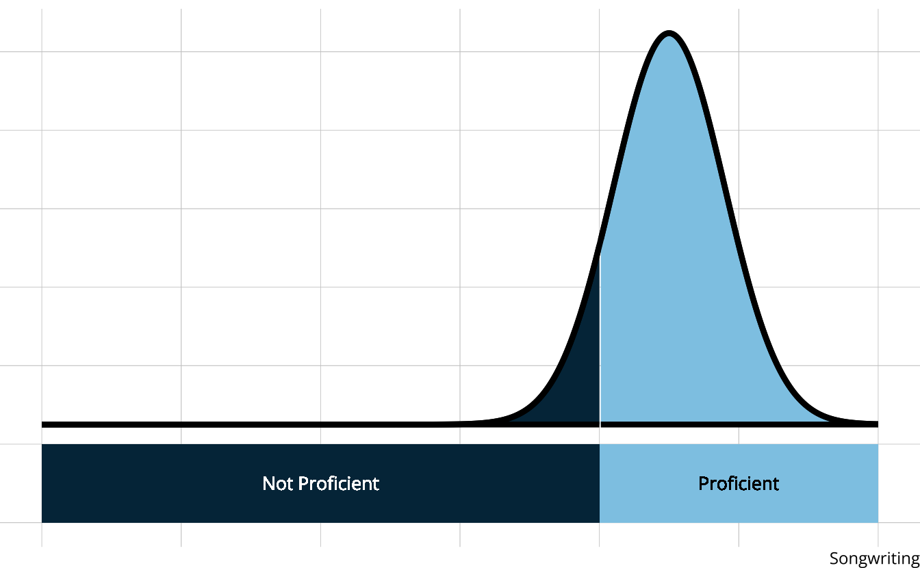
Classification reliability

• Easier to categorize than place along a continuum

• Can set a proficiency threshold to optimize Type 1 or Type 2 errors

When are DCMs appropriate?

Success depends on:

1. Domain definitions
   • What are the attributes we’re trying to measure?
   • Are the attributes measurable (e.g., with assessment items)?
2. Alignment of purpose between assessment and model
   • Is classification the purpose?

Example applications

• Educational measurement: The competencies that student is or is not proficient in
  • Latent knowledge, skills, or understandings
  • Used for tailored instruction and remediation
• Psychiatric assessment: The DSM criteria that an individual meets
  • Broader diagnosis of a disorder

When are DCMs not appropriate?

• When the goal is to place individuals on a scale

• DCMs do not distinguish within classes

	songwriting	production	vocals

Conceptual foundation summary

• DCMs are psychometric models designed to classify
  • We can define our attributes in any way that we choose
  • Items depend on the attribute definitions
  • Classifications are probabilistic

• DCMs provide valuable information with more feasible data demands than other psychometric models
  • Higher reliability than IRT/MIRT models
  • Complex item structures possible
  • Criterion-referenced interpretations
  • Alignment of assessment goals and psychometric model

Statistical foundations

Statistical foundation

• Latent class models use responses to probabilistically place individuals into latent classes

• DCMs are confirmatory latent class models

  • Latent classes specified a priori as attribute profiles
  • Q-matrix specifies item-attribute structure
  • Person parameters are attribute proficiency probabilities

Terminology

• Respondents (r): The individuals from whom behavioral data are collected

  • For today, this is dichotomous assessment item responses
  • Not limited to only item responses in practice

• Items (i): Assessment questions used to classify/diagnose respondents

• Attributes (a): Unobserved latent categorical characteristics underlying the behaviors (i.e., diagnostic status)

  • Latent variables

Attribute profiles

• With binary attributes, there are 2^A possible profiles

• Example 3-attribute assessment:

[0, 0, 0]
[1, 0, 0]
[0, 1, 0]
[0, 0, 1]
[1, 1, 0]
[1, 0, 1]
[0, 1, 1]
[1, 1, 1]

DCMs as latent class models

\[ \color{#D55E00}{P(X_r=x_r)} = \sum_{c=1}^C\color{#009E73}{\nu_c} \prod_{i=1}^I\color{#56B4E9}{\pi_{ic}^{x_{ir}}(1-\pi_{ic})^{1 - x_{ir}}} \]

Observed data: Probability of observing examinee r's item reponses

Structural component: Proportion of examinees in each class

Measurement component: Product of item response probabilities

Structural models

\[ \color{#D55E00}{P(X_r=x_r)} = \sum_{c=1}^C\color{#009E73}{\nu_c} \prod_{i=1}^I\color{#56B4E9}{\pi_{ic}^{x_{ir}}(1-\pi_{ic})^{1 - x_{ir}}} \]

Structural component: Proportion of examinees in each class

• Prevalence of each class in the population
  • ν₁ + ν₂ + … + ν_c = 1
• Typically unconstrained
  • Independent attributes (Lee, 2017)
  • Log-linear structural models (Rupp et al., 2010)

Measurement models

\[ \color{#D55E00}{P(X_r=x_r)} = \sum_{c=1}^C\color{#009E73}{\nu_c} \prod_{i=1}^I\color{#56B4E9}{\pi_{ic}^{x_{ir}}(1-\pi_{ic})^{1 - x_{ir}}} \]

Measurement component: Product of item response probabilities

• Traditional psychometrics: Item response theory, classical test theory
  • A single, unidimensional construct
  • Student results estimated on a continuum
  • Performance on individual items determined by an “item characteristic curve”
• DCMs: Many different options

Diagnostic assessment items

• Can be multidimensional

• No continuum of student achievement

• Categorical constructs

  • Usually binary (e.g., master/nonmaster, proficient/not proficient)

DCM measurement models

• Items can measure one or both attributes

• Different DCMs define π_ic in different ways

  • Each DCM makes different assumptions about how attributes proficiencies combine/interact to produce an item response

• Item characteristic bar charts

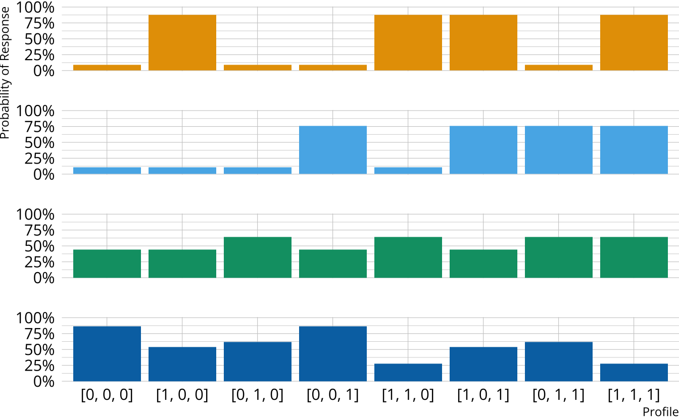
Loglinear cognitive diagnostic model (LCDM)

• Henson et al. (2009)

• Different response probabilities for each class (partially compensatory)

• This will be our focus

Simple structure LCDM

Item measures only 1 attribute

\[ \text{logit}(X_i = 1) = \color{#D7263D}{\lambda_{i,0}} + \color{#219EBC}{\lambda_{i,1(1)}}\color{#009E73}{\alpha} \]

λ_i,0: Log-odds when not proficient

λ_i,1(1): Increase in log-odds when proficient

α: Attribute proficiency status (either 0 or 1)

Subscript notation

λ_i,e(α1)

• i = The item to which the parameter belongs

• e = The level of the effect
  • 0 = intercept
  • 1 = main effect
  • 2 = two-way interaction
  • 3 = three-way interaction
  • Etc.

• (α₁,…) = The attributes to which the effect applies
  • The same number of attributes as listed in subscript 2

Complex structure LCDM

Item measures multiple attributes

\[ \text{logit}(X_i = 1) = \color{#D7263D}{\lambda_{i,0}} + \color{#4B3F72}{\lambda_{i,1(1)}\alpha_1} + \color{#9589BE}{\lambda_{i,1(2)}\alpha_2} + \color{#219EBC}{\lambda_{i,2(1,2)}\alpha_1\alpha_2} \]

Log-odds when proficient in neither attribute

Increase in log-odds when proficient in attribute 1

Increase in log-odds when proficient in attribute 2

Change in log-odds when proficient in both attributes

Defining DCM structures

• Attribute and item relationships are defined in the Q-matrix

• Q-matrix

  • I \(\times\) A matrix
  • 0 = Attribute is not measured by the item
  • 1 = Attribute is measured by the item

The LCDM as a general DCM

• So called “general” DCM because the LCDM subsumes other DCMs

• Constraints on item parameters make LCDM equivalent to other DCMs (e.g., DINA and DINO)

From model parameters to respondents

• Respondent estimates come from combining the estimated model parameters with the response data

• For DCMs, a similar process to that for IRT

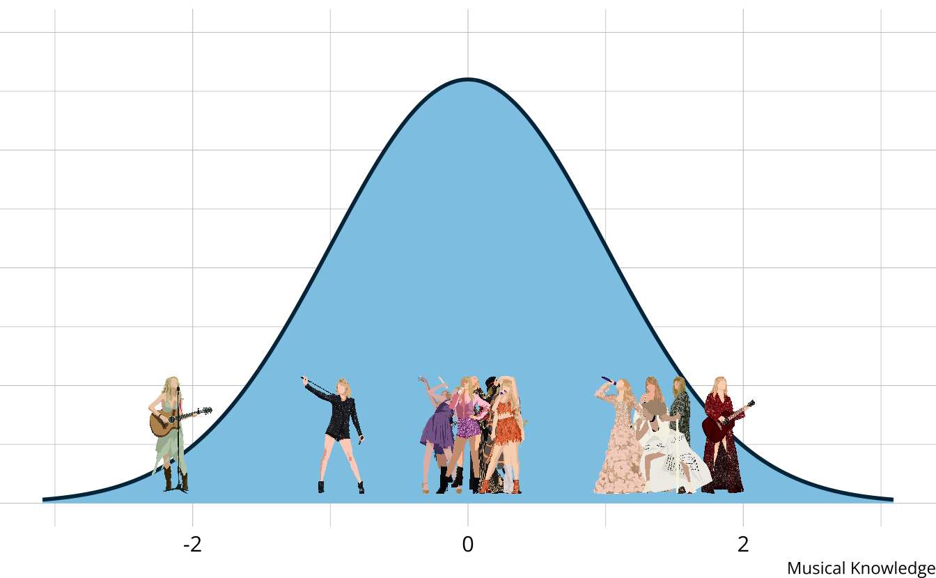
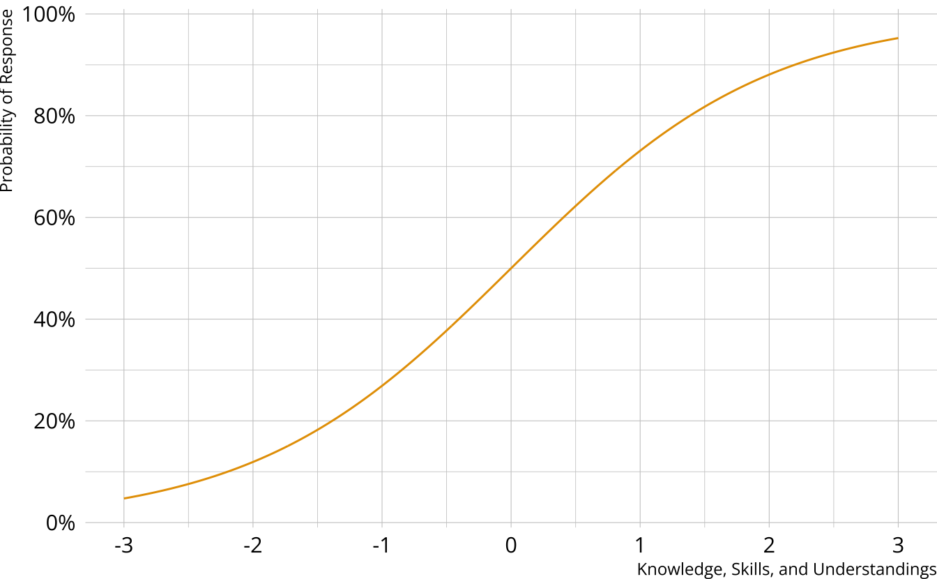
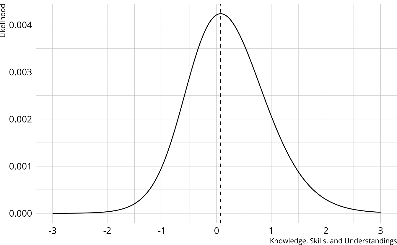
IRT respondent estimates

• Multiply the ICCs together

  • Multiply the response probabilities together for each value of the trait

• Student estimate is the peak of the curve

• Spread of the curve represents uncertainty in estimate

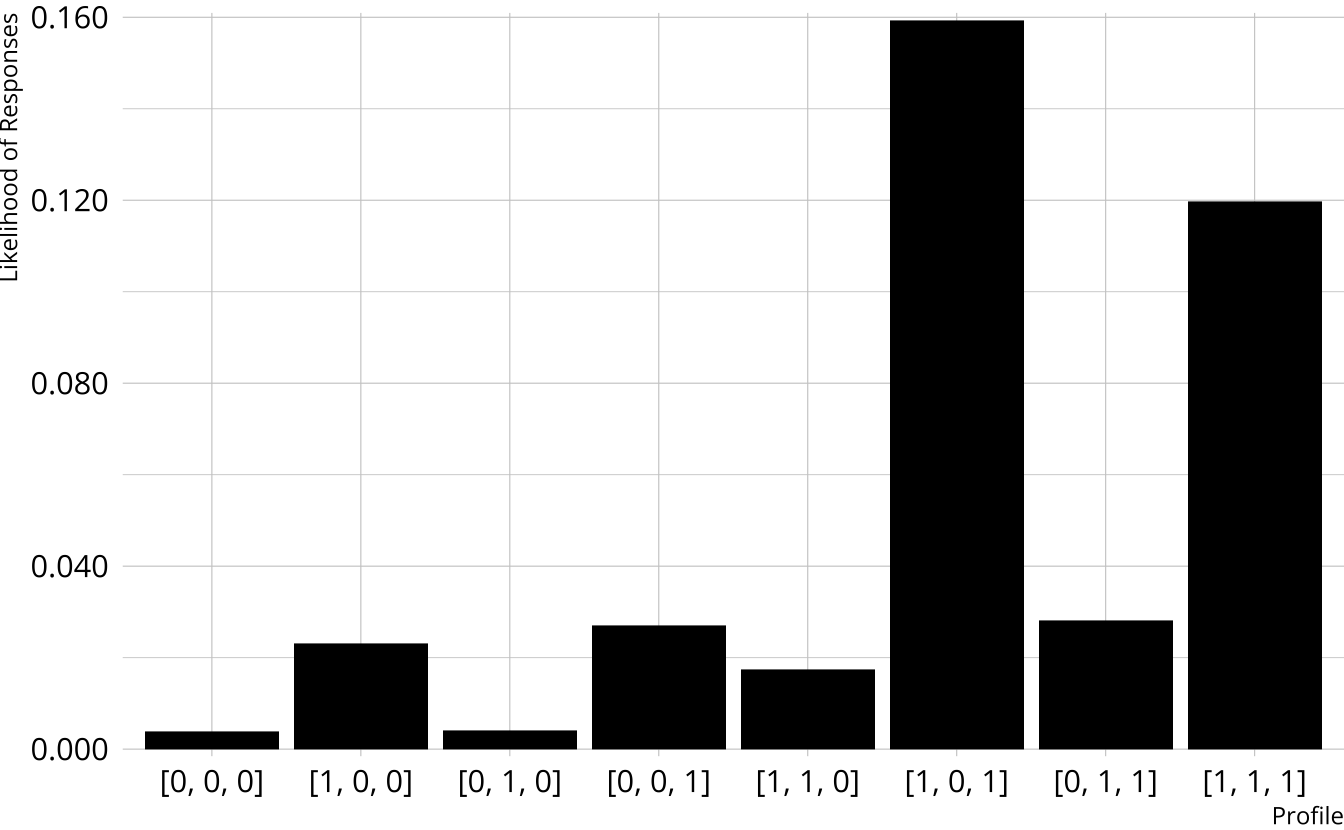
DCM respondent estimates

• Multiply the response probabilities together for each class

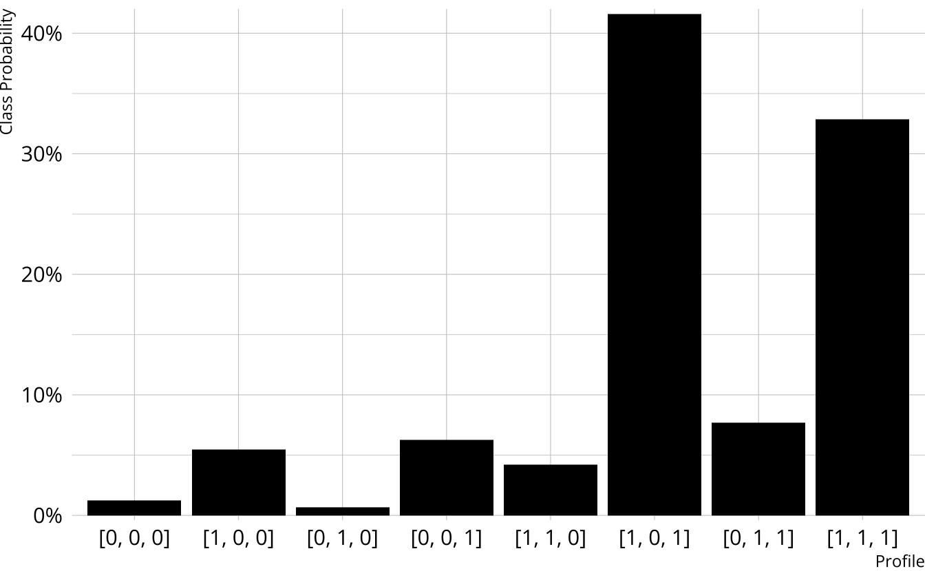
• Multiply the item response likelihoods by structural parameters

• Class probabilities are the class likelihoods divided by the total likelihood

From class to attribute probabilities

• For each attribute, sum the class probabilities where that attribute is present

Songwriting: 84.2%

Production: 45.4%

Vocals: 88.4%

songwriting	production	vocals	probability
0	0	0	0.012
1	0	0	0.055
0	1	0	0.007
0	0	1	0.062
1	1	0	0.042
1	0	1	0.416
0	1	1	0.077
1	1	1	0.328
			0.842

songwriting	production	vocals	probability
0	0	0	0.012
1	0	0	0.055
0	1	0	0.007
0	0	1	0.062
1	1	0	0.042
1	0	1	0.416
0	1	1	0.077
1	1	1	0.328
			0.454

songwriting	production	vocals	probability
0	0	0	0.012
1	0	0	0.055
0	1	0	0.007
0	0	1	0.062
1	1	0	0.042
1	0	1	0.416
0	1	1	0.077
1	1	1	0.328
			0.884

The rest of today

• Estimating DCMs with Stan and measr

• Evaluating DCMs with measr

Diagnostic classification models

A brief introduction

https://learn.r-dcm.org