Evaluating diagnostic
classification models

With Stan and measr

W. Jake Thompson, Ph.D.

Model evaluation

Absolute fit: How well does the model represent the observed data?
- Model-level
- Item-level
Relative fit: How do multiple models compare to each other?
Reliability: How consistent and accurate are the classifications?

Absolute model fit

Model-level absolute fit

Limited information indices based on parameter point estimates
- M₂ statistic (Liu et al., 2016)
Posterior predictive model checks (PPMCs)

Calculating limited information indices

Estimates model fit using univariate and bivariate item relationships
p-values less than .05 indicate poor fit

fit_m2(ecpe_lcdm)
#> # A tibble: 1 × 8
#>      m2    df     pval  rmsea ci_lower ci_upper `90% CI`          srmsr
#>   <dbl> <int>    <dbl>  <dbl>    <dbl>    <dbl> <chr>             <dbl>
#> 1  513.   325 1.18e-10 0.0141   0.0117   0.0164 [0.0117, 0.0164] 0.0312

Also includes the root mean square error of approximation (RMSEA) and the standardized root mean square residual (SRMSR)

Exercise 1

Open evaluation.Rmd and run the setup chunk.
Calculate the M₂ statistic for the ROAR-PA LCDM model
Does the model fit the data?

fit_m2(roarpa_lcdm)
#> # A tibble: 1 × 8
#>      m2    df  pval rmsea ci_lower ci_upper `90% CI` srmsr
#>   <dbl> <int> <dbl> <dbl>    <dbl>    <dbl> <chr>    <dbl>
#> 1 1405.  1532 0.991     0        0        0 [0, 0]   0.107

The null hypothesis is that our model fits the data
- p-values > .05 indicate acceptable model fit

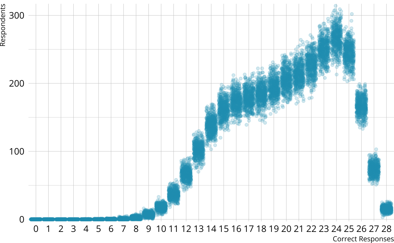
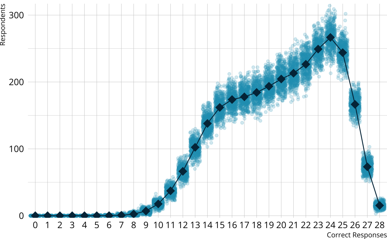
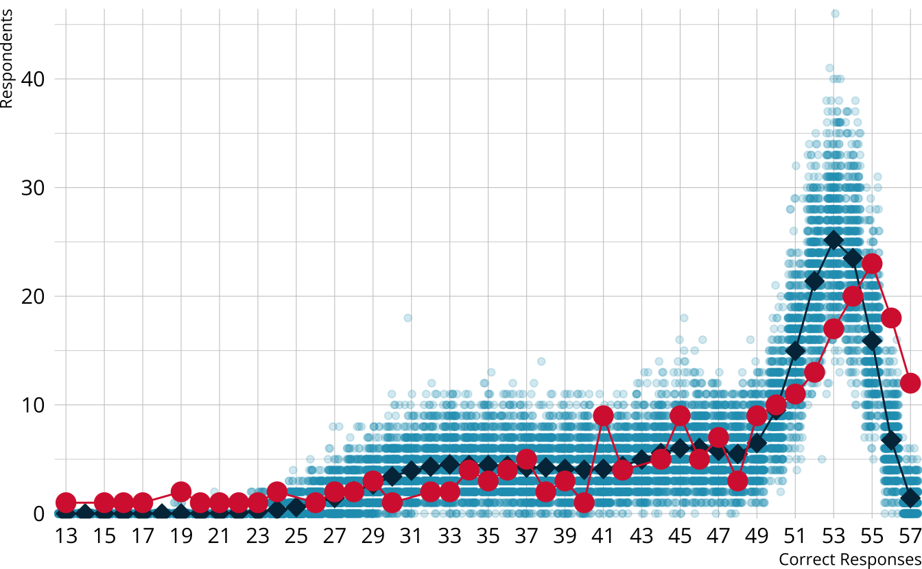
PPMC: Raw score distribution

For each iteration, calculate the total number of respondents at each score point

Calculate the expected number of respondents at each score point

Calculate the observed number of respondents at each score point

Scatter plot showing the number of respondents at each score point in each iteration.

Scatter plot showing the number of respondents at each score point in each iteration with the average number of respondents overlayed.

Scatter plot showing the number of respondents at each score point in each iteration with the average and observed number of respondents overlayed.

PPMC: \(\chi^2\)

Calculate a \(\chi^2\)-like statistic comparing the number of respondents at each score point in each iteration to the expectation

Calculate the \(\chi^2\) value comparing the observed data to the expectation

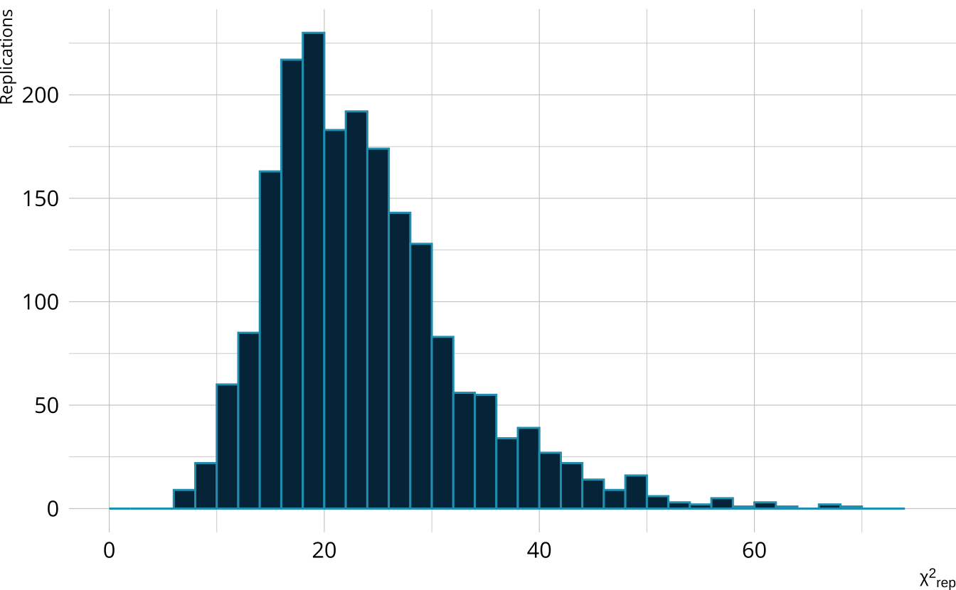
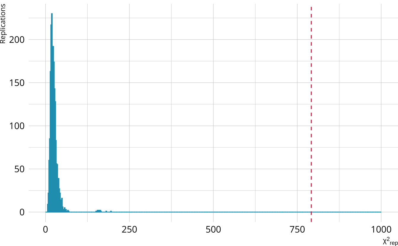
Histogram of the chi-square values from each iteration.

Histogram of the chi-square values from each iteration with a dashed vertical line indicating the value from the observed data.

PPMC: ppp

Calculate the proportion of iterations where the \(\chi^2\)-like statistic from replicated data set exceeds the observed data statistic
- Posterior predictive p-value (ppp)
Very high values (e.g., >.975) or very low values (e.g., <.025) indicate our observed value is far in the tails of what the model would predict
- Poor model fit
Ideally, we’d like ppp values close to .5

PPMCs with measr

fit_ppmc(ecpe_lcdm, model_fit = "raw_score")
#> $ppmc_raw_score
#> # A tibble: 1 × 5
#>   obs_chisq ppmc_mean `2.5%` `97.5%`    ppp
#>       <dbl>     <dbl>  <dbl>   <dbl>  <dbl>
#> 1      792.      25.7   10.7    48.8 0.0005

Exercise 2

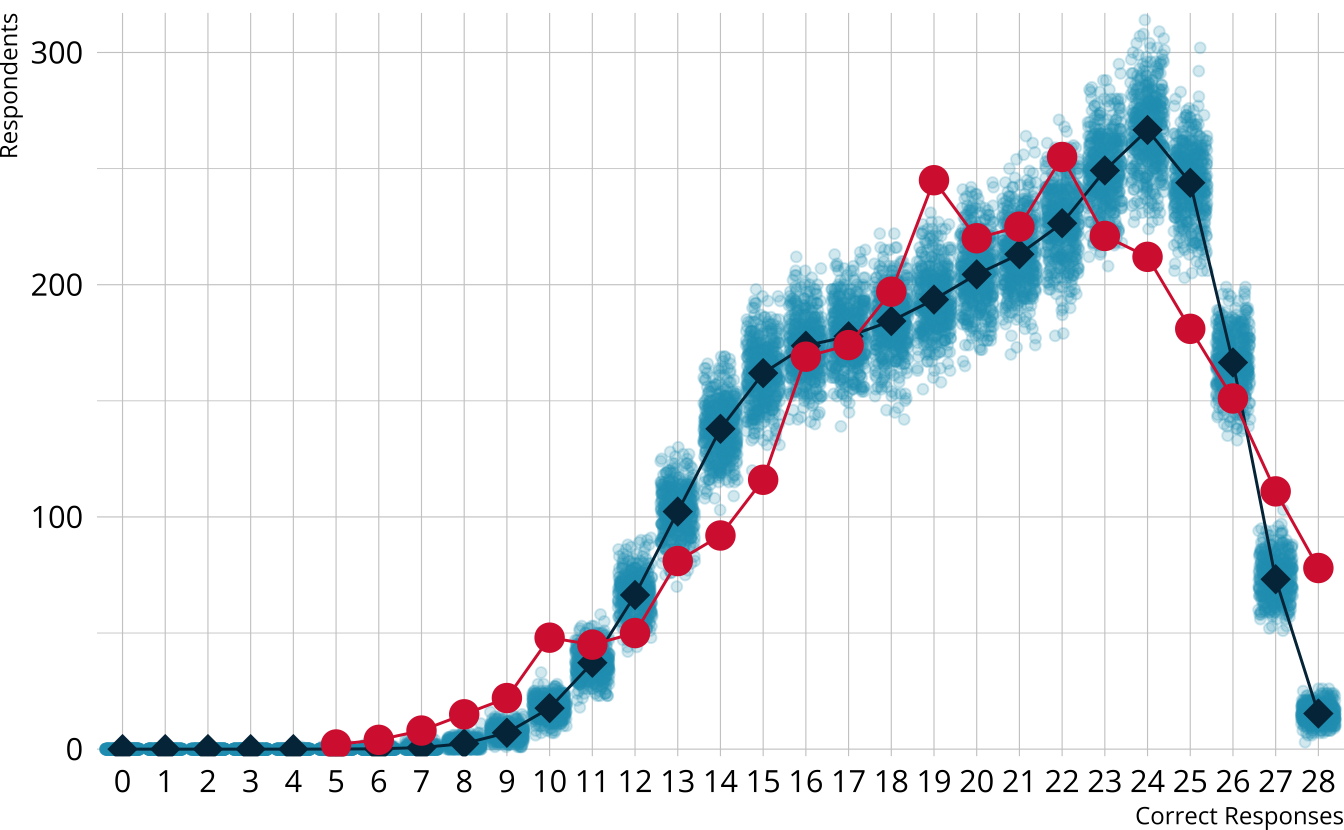
Calculate the raw score PPMC for the ROAR-PA LCDM
Does the model fit the observed data?

fit_ppmc(roarpa_lcdm, model_fit = "raw_score")
#> $ppmc_raw_score
#> # A tibble: 1 × 5
#>   obs_chisq ppmc_mean `2.5%` `97.5%`   ppp
#>       <dbl>     <dbl>  <dbl>   <dbl> <dbl>
#> 1    31865.      45.3   22.0    99.6     0

The ppp value is <.001
Model fit appears to be poor.
Why the difference from the M₂ conclusion?

ROAR-PA raw score distribution

Model is underestimating the number of students with the highest scores
M₂ is limited information—we may miss aspects of the data that come from higher order interactions between items

Item-level fit

Diagnose problems with model-level
Identify particular items that may not be performing as expected
Identify potential dimensionality issues

Item-level fit with measr

Currently support three measures of item-level fit using PPMCs:
- Overall item p-values
- Conditional probability of each class providing a correct response (\(\pi\) matrix)
- Item pair odds ratios

Calculating item-level fit

fit_ppmc(ecpe_lcdm, item_fit = "odds_ratio")
#> $ppmc_odds_ratio
#> # A tibble: 378 × 7
#>    item_1 item_2 obs_or ppmc_mean `2.5%` `97.5%`   ppp
#>    <chr>  <chr>   <dbl>     <dbl>  <dbl>   <dbl> <dbl>
#>  1 E1     E2       1.61      1.42   1.11    1.78 0.140
#>  2 E1     E3       1.42      1.56   1.27    1.86 0.810
#>  3 E1     E4       1.58      1.40   1.15    1.70 0.114
#>  4 E1     E5       1.68      1.47   1.10    1.89 0.159
#>  5 E1     E6       1.64      1.38   1.07    1.77 0.085
#>  6 E1     E7       1.99      1.89   1.55    2.30 0.286
#>  7 E1     E8       1.54      1.59   1.18    2.06 0.574
#>  8 E1     E9       1.18      1.32   1.08    1.60 0.871
#>  9 E1     E10      1.82      1.69   1.37    2.04 0.220
#> 10 E1     E11      1.61      1.73   1.40    2.08 0.736
#> # ℹ 368 more rows

Extracting item-level fit

measr_extract(ecpe_lcdm, "ppmc_pvalue")
#> # A tibble: 28 × 7
#>    item_id obs_pvalue ppmc_mean `2.5%` `97.5%` samples          ppp
#>    <fct>        <dbl>     <dbl>  <dbl>   <dbl> <named list>   <dbl>
#>  1 E1           0.803     0.810  0.786   0.827 <dbl [2,000]> 0.798 
#>  2 E2           0.830     0.831  0.815   0.846 <dbl [2,000]> 0.554 
#>  3 E3           0.579     0.553  0.531   0.591 <dbl [2,000]> 0.0885
#>  4 E4           0.706     0.697  0.680   0.716 <dbl [2,000]> 0.167 
#>  5 E5           0.887     0.886  0.873   0.900 <dbl [2,000]> 0.419 
#>  6 E6           0.854     0.854  0.839   0.868 <dbl [2,000]> 0.512 
#>  7 E7           0.721     0.708  0.690   0.733 <dbl [2,000]> 0.118 
#>  8 E8           0.898     0.900  0.888   0.912 <dbl [2,000]> 0.626 
#>  9 E9           0.702     0.695  0.675   0.719 <dbl [2,000]> 0.239 
#> 10 E10          0.658     0.670  0.640   0.690 <dbl [2,000]> 0.844 
#> # ℹ 18 more rows

measr_extract(ecpe_lcdm, "ppmc_pvalue_flags")
#> # A tibble: 0 × 7
#> # ℹ 7 variables: item_id <fct>, obs_pvalue <dbl>, ppmc_mean <dbl>, 2.5% <dbl>,
#> #   97.5% <dbl>, samples <named list>, ppp <dbl>

measr_extract(ecpe_lcdm, "ppmc_conditional_prob_flags")
#> # A tibble: 142 × 8
#>    item_id class   obs_cond_pval ppmc_mean `2.5%` `97.5%` samples          ppp
#>    <chr>   <chr>           <dbl>     <dbl>  <dbl>   <dbl> <named list>   <dbl>
#>  1 E1      [0,0,0]         0.701     0.695  0.672   0.699 <dbl [2,000]> 0.0055
#>  2 E1      [1,0,0]         0.664     0.822  0.795   0.827 <dbl [2,000]> 1     
#>  3 E1      [0,0,1]         0.582     0.695  0.672   0.699 <dbl [2,000]> 1     
#>  4 E1      [1,1,0]         1         0.941  0.930   0.942 <dbl [2,000]> 0     
#>  5 E1      [1,0,1]         0.617     0.822  0.795   0.827 <dbl [2,000]> 1     
#>  6 E1      [0,1,1]         0.854     0.813  0.791   0.819 <dbl [2,000]> 0     
#>  7 E1      [1,1,1]         0.928     0.941  0.930   0.942 <dbl [2,000]> 0.98  
#>  8 E2      [1,0,0]         0.803     0.741  0.730   0.744 <dbl [2,000]> 0     
#>  9 E2      [0,0,1]         0.712     0.741  0.730   0.744 <dbl [2,000]> 0.991 
#> 10 E2      [1,1,0]         1         0.908  0.907   0.913 <dbl [2,000]> 0     
#> # ℹ 132 more rows

measr_extract(ecpe_lcdm, "ppmc_odds_ratio_flags")
#> # A tibble: 78 × 8
#>    item_1 item_2 obs_or ppmc_mean `2.5%` `97.5%` samples          ppp
#>    <chr>  <chr>   <dbl>     <dbl>  <dbl>   <dbl> <named list>   <dbl>
#>  1 E1     E17      2.02      1.50   1.13    1.94 <dbl [2,000]> 0.0155
#>  2 E1     E26      1.61      1.29   1.05    1.57 <dbl [2,000]> 0.014 
#>  3 E1     E28      1.86      1.43   1.13    1.77 <dbl [2,000]> 0.0075
#>  4 E2     E4       1.73      1.35   1.09    1.65 <dbl [2,000]> 0.0055
#>  5 E2     E5       1.84      1.40   1.03    1.83 <dbl [2,000]> 0.024 
#>  6 E2     E6       1.72      1.33   1.00    1.72 <dbl [2,000]> 0.024 
#>  7 E2     E14      1.64      1.24   1.01    1.51 <dbl [2,000]> 0.002 
#>  8 E2     E15      1.92      1.45   1.07    1.90 <dbl [2,000]> 0.02  
#>  9 E4     E5       2.81      2.06   1.63    2.58 <dbl [2,000]> 0.0065
#> 10 E4     E8       2.14      1.48   1.13    1.90 <dbl [2,000]> 0.0005
#> # ℹ 68 more rows

Patterns of item-level misfit

measr_extract(ecpe_lcdm, "ppmc_conditional_prob_flags") |>
  count(class, name = "flags") |>
  left_join(measr_extract(ecpe_lcdm, "strc_param"), by = join_by(class)) |>
  arrange(desc(flags))
#> # A tibble: 7 × 6
#>   class   flags morphosyntactic cohesive lexical         estimate
#>   <chr>   <int>           <int>    <int>   <int>       <rvar[1d]>
#> 1 [1,0,1]    27               1        0       1  0.020 ± 0.00097
#> 2 [1,0,0]    26               1        0       0  0.018 ± 0.00198
#> 3 [0,0,1]    25               0        0       1  0.133 ± 0.00517
#> 4 [1,1,0]    23               1        1       0  0.015 ± 0.00253
#> 5 [0,1,1]    21               0        1       1  0.154 ± 0.00909
#> 6 [0,0,0]    12               0        0       0  0.291 ± 0.00588
#> 7 [1,1,1]     8               1        1       1  0.350 ± 0.00487

Exercise 3

Calculate PPMCs for the conditional probabilities and odds ratios for the ROAR-PA model
What do the results tell us about the model?

Conditional probabilities
Odds ratios

measr_extract(roarpa_lcdm, "ppmc_conditional_prob_flags") |>
  count(class, name = "flags") |>
  left_join(measr_extract(roarpa_lcdm, "strc_param"), by = join_by(class)) |>
  arrange(desc(flags))
#> # A tibble: 8 × 6
#>   class   flags   lsm   del   fsm        estimate
#>   <chr>   <int> <int> <int> <int>      <rvar[1d]>
#> 1 [1,0,0]    54     1     0     0  0.011 ± 0.0083
#> 2 [1,0,1]    42     1     0     1  0.042 ± 0.0162
#> 3 [1,1,0]    39     1     1     0  0.037 ± 0.0151
#> 4 [0,0,1]    38     0     0     1  0.059 ± 0.0198
#> 5 [0,1,0]    31     0     1     0  0.047 ± 0.0169
#> 6 [0,1,1]    24     0     1     1  0.099 ± 0.0228
#> 7 [0,0,0]    11     0     0     0  0.158 ± 0.0269
#> 8 [1,1,1]     2     1     1     1  0.546 ± 0.0400

measr_extract(roarpa_lcdm, "ppmc_odds_ratio_flags")
#> # A tibble: 164 × 8
#>    item_1 item_2 obs_or ppmc_mean `2.5%` `97.5%` samples          ppp
#>    <chr>  <chr>   <dbl>     <dbl>  <dbl>   <dbl> <named list>   <dbl>
#>  1 fsm_01 lsm_07  7.20       2.84  0.956    6.59 <dbl [2,000]> 0.016 
#>  2 fsm_01 lsm_08  5.84       2.47  0.839    5.72 <dbl [2,000]> 0.023 
#>  3 fsm_01 lsm_19  0.349      2.44  0.378    6.30 <dbl [2,000]> 0.978 
#>  4 fsm_01 del_09 12.3        3.21  0.731    8.22 <dbl [2,000]> 0.003 
#>  5 fsm_01 del_15  7.81       2.57  0.520    6.49 <dbl [2,000]> 0.0115
#>  6 fsm_04 fsm_11 13.6        4.38  0       13.1  <dbl [2,000]> 0.019 
#>  7 fsm_04 del_01 11          2.31  0        8.20 <dbl [2,000]> 0.012 
#>  8 fsm_04 del_07  7.75     Inf     0        6.44 <dbl [2,000]> 0.0105
#>  9 fsm_04 del_09 14.0      Inf     0        8.99 <dbl [2,000]> 0.0045
#> 10 fsm_04 del_16  5.08       1.80  0        5.00 <dbl [2,000]> 0.0235
#> # ℹ 154 more rows

Relative model fit

Model comparisons

Doesn’t give us information whether or not a model fits the data, only compares competing models to each other
- Should be evaluated in conjunction with absolute model fit
Implemented with the loo package
- PSIS-LOO (Vehtari, 2017)
- WAIC (Watanabe, 2010)

Relative fit with measr

loo(ecpe_lcdm)
#> 
#> Computed from 2000 by 2922 log-likelihood matrix.
#> 
#>          Estimate    SE
#> elpd_loo -42794.9 226.8
#> p_loo        23.4   0.4
#> looic     85589.7 453.7
#> ------
#> MCSE of elpd_loo is NA.
#> MCSE and ESS estimates assume independent draws (r_eff=1).
#> 
#> Pareto k diagnostic values:
#>                          Count Pct.    Min. ESS
#> (-Inf, 0.7]   (good)      749  25.6%   1897    
#>    (0.7, 1]   (bad)        13   0.4%   <NA>    
#>    (1, Inf)   (very bad) 2160  73.9%   <NA>    
#> See help('pareto-k-diagnostic') for details.

waic(ecpe_lcdm)
#> 
#> Computed from 2000 by 2922 log-likelihood matrix.
#> 
#>           Estimate    SE
#> elpd_waic -42794.8 226.8
#> p_waic        23.3   0.4
#> waic       85589.5 453.7

Comparing models

First, we need another model to compare

ecpe_dina_spec <- dcm_specify(
  qmatrix = ecpe_qmatrix,
  identifier = "item_id",
  measurement_model = dina(),
  structural_model = unconstrained()
)

ecpe_dina <- dcm_estimate(
  ecpe_dina_spec,
  data = ecpe_data,
  identifier = "resp_id",
  method = "pathfinder",
  backend = "cmdstanr",
  single_path_draws = 1000,
  num_paths = 10,
  draws = 2000,
  file = here("materials", "slides", "fits", "ecpe-dina-uncst")
)

`loo_compare()`

loo_compare(ecpe_lcdm, ecpe_dina)
#>           elpd_diff se_diff
#> ecpe_lcdm    0.0       0.0 
#> ecpe_dina -128.7      21.6

LCDM is the preferred model
- Preferred does not imply “good”
- Remember, the LCDM showed poor absolute fit
Difference is much larger than the standard error of the difference
- Approximate threshold: Absolute difference is greater than 2.5 × standard error of the difference (Bengio & Grandvalet, 2004)

Exercise 4

Estimate a DINA model for the ROAR-PA data
Use loo_compare() to compare the LCDM and DINA models
- What do the findings tell us?
- Can you explain the results?

Estimate DINA model
Compare models

roarpa_dina_spec <- dcm_specify(
  qmatrix = roarpa_qmatrix,
  identifier = "item",
  measurement_model = dina(),
  structural_model = unconstrained()
)

roarpa_dina <- dcm_estimate(
  roarpa_dina_spec,
  data = roarpa_data,
  identifier = "id",
  method = "variational",
  backend = "rstan",
  seed = 19891213,
  file = here("materials", "slides", "fits", "roarpa-dina-uncst")
)

loo_compare(roarpa_lcdm, roarpa_dina, criterion = "loo")
#>             elpd_diff se_diff
#> roarpa_lcdm    0.0       0.0 
#> roarpa_dina -104.2      42.9

loo_compare(roarpa_lcdm, roarpa_dina, criterion = "waic")
#>             elpd_diff se_diff
#> roarpa_lcdm    0.0       0.0 
#> roarpa_dina -104.5      42.9

Reliability

Reliability methods

Reporting reliability depends on how results are estimated and reported
Reliability for:
- Profile-level classification
- Attribute-level classification
- Attribute-level probability of proficiency

Reliability with measr

reliability(ecpe_lcdm)
#> $pattern_reliability
#>       p_a       p_c 
#> 0.7357164 0.6525172 
#> 
#> $map_reliability
#> $map_reliability$accuracy
#> # A tibble: 3 × 8
#>   attribute         acc lambda_a kappa_a youden_a tetra_a  tp_a  tn_a
#>   <chr>           <dbl>    <dbl>   <dbl>    <dbl>   <dbl> <dbl> <dbl>
#> 1 morphosyntactic 0.896    0.734   0.789    0.780   0.943 0.864 0.916
#> 2 cohesive        0.851    0.678   0.700    0.699   0.891 0.870 0.829
#> 3 lexical         0.916    0.752   0.603    0.805   0.959 0.945 0.859
#> 
#> $map_reliability$consistency
#> # A tibble: 3 × 10
#>   attribute       consist lambda_c kappa_c youden_c tetra_c  tp_c  tn_c gammak
#>   <chr>             <dbl>    <dbl>   <dbl>    <dbl>   <dbl> <dbl> <dbl>  <dbl>
#> 1 morphosyntactic   0.818    0.534   0.710    0.618   0.828 0.767 0.850  0.852
#> 2 cohesive          0.800    0.560   0.688    0.597   0.807 0.817 0.780  0.788
#> 3 lexical           0.864    0.583   0.635    0.690   0.890 0.899 0.791  0.880
#> # ℹ 1 more variable: pc_prime <dbl>
#> 
#> 
#> $eap_reliability
#> # A tibble: 3 × 5
#>   attribute       rho_pf rho_bs rho_i rho_tb
#>   <chr>            <dbl>  <dbl> <dbl>  <dbl>
#> 1 morphosyntactic  0.706  0.689 0.577  0.885
#> 2 cohesive         0.707  0.574 0.506  0.785
#> 3 lexical          0.776  0.731 0.588  0.916

Profile-level classification

Profile-level probabilities
Profile-level classifications
Profile reliability

measr_extract(ecpe_lcdm, "class_prob")
#> # A tibble: 2,922 × 9
#>    resp_id `[0,0,0]` `[1,0,0]` `[0,1,0]` `[0,0,1]` `[1,1,0]` `[1,0,1]` `[0,1,1]`
#>    <chr>       <dbl>     <dbl>     <dbl>     <dbl>     <dbl>     <dbl>     <dbl>
#>  1 1         5.21e-6   1.27e-4   4.15e-7  0.00127  0.000118   0.0472     0.00171
#>  2 2         5.10e-6   1.25e-4   2.20e-7  0.00352  0.0000636  0.130      0.00156
#>  3 3         5.59e-6   1.87e-5   2.23e-6  0.00315  0.0000902  0.00959    0.0211 
#>  4 4         2.02e-7   4.94e-6   8.07e-8  0.000264 0.0000230  0.00981    0.00178
#>  5 5         6.73e-4   9.61e-3   2.69e-4  0.00112  0.0450     0.00920    0.00752
#>  6 6         1.93e-6   1.70e-5   7.70e-7  0.000840 0.0000795  0.00977    0.00566
#>  7 7         1.93e-6   1.70e-5   7.70e-7  0.000840 0.0000795  0.00977    0.00566
#>  8 8         2.62e-2   7.33e-5   1.09e-3  0.571    0.0000203  0.000295   0.400  
#>  9 9         4.77e-5   3.05e-4   1.91e-5  0.00606  0.00147    0.00935    0.0408 
#> 10 10        2.60e-1   5.98e-1   2.02e-3  0.0331   0.0556     0.0161     0.00432
#> # ℹ 2,912 more rows
#> # ℹ 1 more variable: `[1,1,1]` <dbl>

measr_extract(ecpe_lcdm, "class_prob") |>
  pivot_longer(-resp_id, names_to = "profile", values_to = "prob") |>
  slice_max(order_by = prob, by = resp_id)
#> # A tibble: 2,922 × 3
#>    resp_id profile  prob
#>    <chr>   <chr>   <dbl>
#>  1 1       [1,1,1] 0.950
#>  2 2       [1,1,1] 0.864
#>  3 3       [1,1,1] 0.966
#>  4 4       [1,1,1] 0.988
#>  5 5       [1,1,1] 0.927
#>  6 6       [1,1,1] 0.984
#>  7 7       [1,1,1] 0.984
#>  8 8       [0,0,1] 0.571
#>  9 9       [1,1,1] 0.942
#> 10 10      [1,0,0] 0.598
#> # ℹ 2,912 more rows

measr_extract(ecpe_lcdm, "pattern_reliability")
#> # A tibble: 1 × 2
#>   accuracy consistency
#>      <dbl>       <dbl>
#> 1    0.736       0.653

Estimating classification consistency and accuracy for cognitive diagnostic assessment (Cui et al., 2012)

Attribute-level classification

Attribute-level probabilities
Attribute-level classifications
Classification reliability

measr_extract(ecpe_lcdm, "attribute_prob")
#> # A tibble: 2,922 × 4
#>    resp_id morphosyntactic cohesive lexical
#>    <chr>             <dbl>    <dbl>   <dbl>
#>  1 1               0.997     0.951   1.000 
#>  2 2               0.995     0.866   1.000 
#>  3 3               0.976     0.987   1.000 
#>  4 4               0.998     0.990   1.000 
#>  5 5               0.990     0.979   0.944 
#>  6 6               0.993     0.989   1.000 
#>  7 7               0.993     0.989   1.000 
#>  8 8               0.00208   0.403   0.973 
#>  9 9               0.953     0.984   0.998 
#> 10 10              0.701     0.0932  0.0847
#> # ℹ 2,912 more rows

measr_extract(ecpe_lcdm, "attribute_prob") |>
  mutate(across(where(is.double), \(x) as.integer(x > 0.5)))
#> # A tibble: 2,922 × 4
#>    resp_id morphosyntactic cohesive lexical
#>    <chr>             <int>    <int>   <int>
#>  1 1                     1        1       1
#>  2 2                     1        1       1
#>  3 3                     1        1       1
#>  4 4                     1        1       1
#>  5 5                     1        1       1
#>  6 6                     1        1       1
#>  7 7                     1        1       1
#>  8 8                     0        0       1
#>  9 9                     1        1       1
#> 10 10                    1        0       0
#> # ℹ 2,912 more rows

measr_extract(ecpe_lcdm, "classification_reliability")
#> # A tibble: 3 × 3
#>   attribute       accuracy consistency
#>   <chr>              <dbl>       <dbl>
#> 1 morphosyntactic    0.896       0.818
#> 2 cohesive           0.851       0.800
#> 3 lexical            0.916       0.864

Measures of agreement to assess attribute-level classification accuracy and consistency for cognitive diagnostic assessments (Johnson & Sinharay, 2018)

Attribute-level probabilities

Attribute-level probabilities
Probability reliability

measr_extract(ecpe_lcdm, "attribute_prob")
#> # A tibble: 2,922 × 4
#>    resp_id morphosyntactic cohesive lexical
#>    <chr>             <dbl>    <dbl>   <dbl>
#>  1 1               0.997     0.951   1.000 
#>  2 2               0.995     0.866   1.000 
#>  3 3               0.976     0.987   1.000 
#>  4 4               0.998     0.990   1.000 
#>  5 5               0.990     0.979   0.944 
#>  6 6               0.993     0.989   1.000 
#>  7 7               0.993     0.989   1.000 
#>  8 8               0.00208   0.403   0.973 
#>  9 9               0.953     0.984   0.998 
#> 10 10              0.701     0.0932  0.0847
#> # ℹ 2,912 more rows

measr_extract(ecpe_lcdm, "probability_reliability")
#> # A tibble: 3 × 2
#>   attribute       informational
#>   <chr>                   <dbl>
#> 1 morphosyntactic         0.577
#> 2 cohesive                0.506
#> 3 lexical                 0.588

The reliability of the posterior probability of skill attainment in diagnostic classification models (Johnson & Sinharay, 2020)

Exercise 5

Examine the attribute classification indices for the ROAR-PA LCDM.
Which attributes are the most and least reliable?

measr_extract(roarpa_lcdm, "classification_reliability")
#> # A tibble: 3 × 3
#>   attribute accuracy consistency
#>   <chr>        <dbl>       <dbl>
#> 1 lsm          0.982       0.994
#> 2 del          0.963       0.958
#> 3 fsm          0.982       0.994

Evaluating diagnostic classification models

With Stan and measr

https://learn.r-dcm.org