library(dcmdata)

ecpe_data
#> # A tibble: 2,922 × 29
#>    resp_id    E1    E2    E3    E4    E5    E6    E7    E8    E9   E10   E11
#>      <int> <int> <int> <int> <int> <int> <int> <int> <int> <int> <int> <int>
#>  1       1     1     1     1     0     1     1     1     1     1     1     1
#>  2       2     1     1     1     1     1     1     1     1     1     1     1
#>  3       3     1     1     1     1     1     1     0     1     1     1     1
#>  4       4     1     1     1     1     1     1     1     1     1     1     1
#>  5       5     1     1     1     1     1     1     1     1     1     1     1
#>  6       6     1     1     1     1     1     1     1     1     1     1     1
#>  7       7     1     1     1     1     1     1     1     1     1     1     1
#>  8       8     0     1     1     1     1     1     0     1     1     1     0
#>  9       9     1     1     1     1     1     1     1     1     1     1     1
#> 10      10     1     1     1     1     0     0     1     1     1     1     1
#> # ℹ 2,912 more rows
#> # ℹ 17 more variables: E12 <int>, E13 <int>, E14 <int>, E15 <int>, E16 <int>,
#> #   E17 <int>, E18 <int>, E19 <int>, E20 <int>, E21 <int>, E22 <int>,
#> # E23 <int>, E24 <int>, E25 <int>, E26 <int>, E27 <int>, E28 <int>Diagnostic measurement
models
W. Jake Thompson, Ph.D.
Example data
Data for examples
- Examination for the certificate of proficiency in English (ECPE; Templin & Hoffman, 2013)
- 28 items measuring 3 total attributes
- 2,922 respondents
- 3 attributes
- Morphosyntactic rules
- Cohesive rules
- Lexical rules
ECPE data
ECPE Q-matrix
Data for exercises
- Pathways for Instructionally Embedded Assessment (PIE; ATLAS, 2025)
Exercise 1
- Download the exercise files
Open
measurement-models.RmdRun the
setupchunkExplore the PIE field test data and Q-matrix
- How many items are in the data?
- How many respondents are in the data?
- How many attributes are measured?
pie_ft_data
#> # A tibble: 172 × 16
#>    student `00592` `14415` `56400` `64967` `06238` `10231` `54596` `96748`
#>    <chr>     <int>   <int>   <int>   <int>   <int>   <int>   <int>   <int>
#>  1 8978593       1       1       1       1       1       0       1       1
#>  2 5231294       1       1       1       1       1       1       1       1
#>  3 3681220       1       1       1       1       1       1       1       1
#>  4 7763384       1       0       1       1       1       1       1       1
#>  5 1913897       1       1       1       1       1       1       1       1
#>  6 0692477       1       1       1       1       1       1       1       1
#>  7 6961042       1       1       0       1       1       1       1       1
#>  8 4241777       1       1       1       1       1       1       1       1
#>  9 3068583       1       1       1       1       1       1       1       1
#> 10 6607413       1       1       1       1       1       1       1       1
#> # ℹ 162 more rows
#> # ℹ 7 more variables: `97634` <int>, `13080` <int>, `27971` <int>,
#> # `56741` <int>, `63088` <int>, `81175` <int>, `88063` <int>- 15 items
- 172 respondents
pie_ft_qmatrix
#> # A tibble: 15 × 4
#>    task     L1    L2    L3
#>    <chr> <int> <int> <int>
#>  1 00592     1     0     0
#>  2 14415     1     0     0
#>  3 56400     1     0     0
#>  4 64967     1     0     0
#>  5 06238     0     1     0
#>  6 10231     0     1     0
#>  7 54596     0     1     0
#>  8 96748     0     1     0
#>  9 97634     0     1     0
#> 10 13080     0     0     1
#> 11 27971     0     0     1
#> 12 56741     0     0     1
#> 13 63088     0     0     1
#> 14 81175     0     0     1
#> 15 88063 0 0 1- 15 items
- 3 attributes representing levels in a learning pathway
- Level 1 (
L1) - Level 2 (
L2) - Level 3 (
L3)
- Level 1 (
Model specification
Specify a DCM with dcm_specify()
Model estimation
Estimate a DCM with dcm_estimate()
- 1
- Define your model specification
- 2
- Specify your data and ID column (if present)
- 3
- Choose your estimation method and backend
- 4
- Pass additional arguments to the backend
- 5
- Save the model for future efficiency
dcm_estimate() options
method: How to estimate the model- Full posterior sampling with “mcmc”
- Quicker, but more limited “optim”
- Posterior approximation with “variational” (default) or “pathfinder”
- Variational inference does not always converge
- Pathfinder is only available for the cmdstanr backend
...: Additional arguments that are passed to, depending on themethodandbackend
DCM item models
Diagnostic assessment items
Can be multidimensional
No continuum of student achievement
Categorical constructs
- Usually binary (e.g., master/nonmaster, proficient/not proficient)
DCM measurement models
Items can measure one or both attributes
Different DCMs define πic in different ways
- Each DCM makes different assumptions about how attributes proficiencies combine/interact to produce an item response
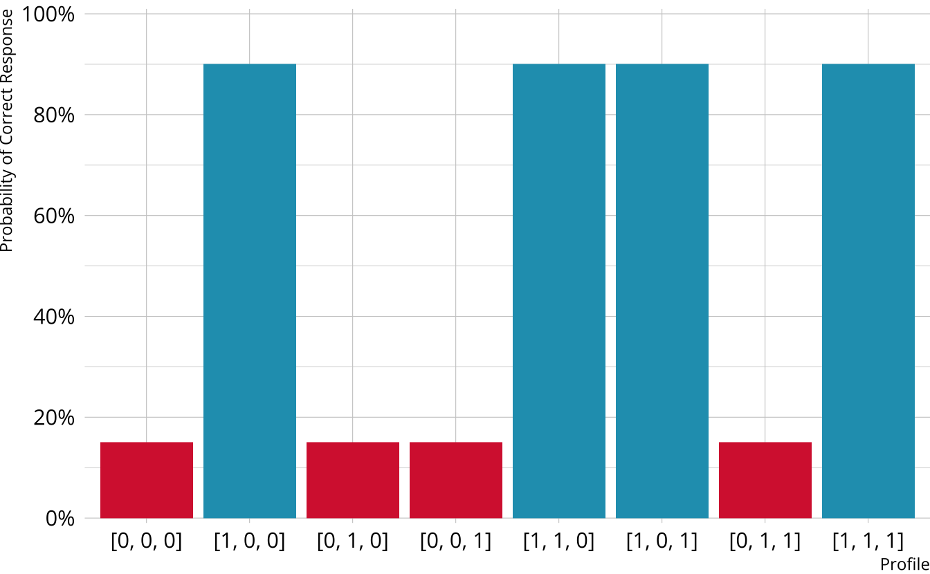
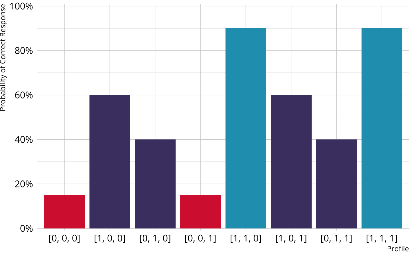
Item characteristic bar charts
Single-attribute DCM item
Item measures just attribute 1
Respondents who are proficient on attribute 1 have high probability of correct response, regardless of other attributes
Multi-attribute items
When items measure multiple attributes, what level of mastery is needed in order to provide a correct response?
Many different types of DCMs that define this probability differently
- Compensatory (e.g., DINO)
- Noncompensatory (e.g., DINA)
- Partially compensatory (e.g., C-RUM)
General diagnostic models (e.g., LCDM)
Each DCM makes different assumptions about how attributes proficiencies combine/interact to produce an item response
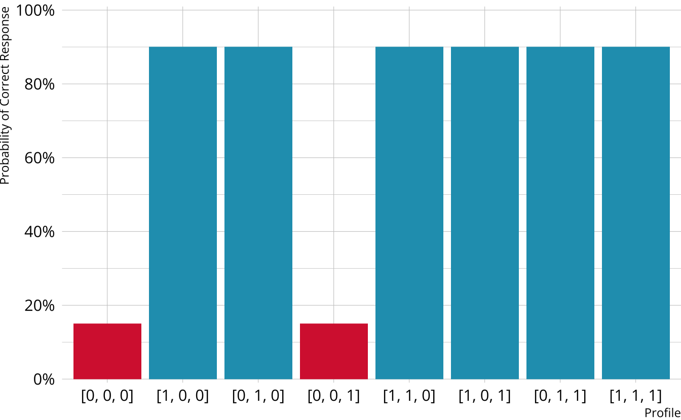
Compensatory DCMs
Item measures attributes 1 and 2
Must be proficient in at least 1 attribute measured by the item to provide a correct response
Deterministic inputs, noisy “or” gate (DINO; Templin & Henson, 2006)
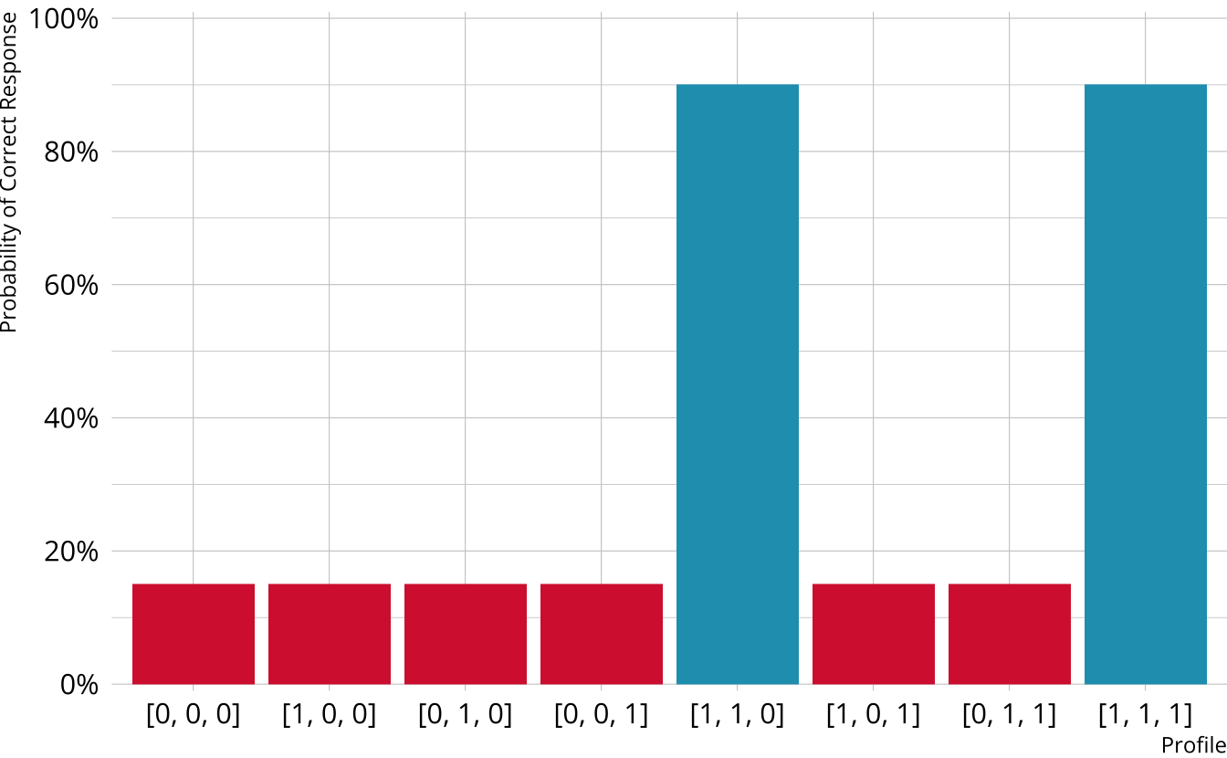
Non-compensatory DCMs
Item measures attributes 1 and 2
Must be proficient in all attributes measured by the item to provide a correct response
Deterministic inputs, noisy “and” gate (DINA; de la Torre & Douglas, 2004)
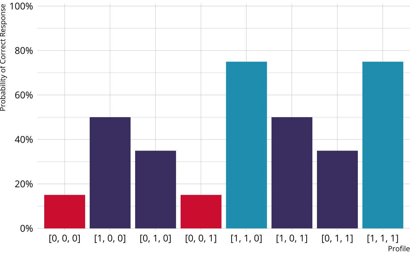
Partially Compensatory DCMs
Separate increases for each acquired attribute
Compensatory reparameterized unified model (C-RUM; Hartz, 2002)
Which DCM to use?
DINO, DINA, and C-RUM are just three of the MANY models that are available
Each model comes with its own set of restrictions, and we typically have to specify a single model that is used for all items (software constraint)
General form diagnostic models
- Flexible; can subsume other more restrictive models
- Again, several possibilities (e.g., G-DINA, GDM, LCDM)
General DCMs
Different response probabilities for each class (partially compensatory)
Log-linear cognitive diagnostic model (LCDM; Henson et al., 2009)
The LCDM as a general DCM
So called “general” DCM because the LCDM subsumes other DCMs
Constraints on item parameters make LCDM equivalent to other DCMs (e.g., DINA and DINO)
- DINA
- Only the intercept and highest-order interaction are non-0
- DINO
- All main effects are equal
- All two-way interactions are -1 \(\times\) main effect
- All three-way interactions are -1 \(\times\) two-way interaction (i.e., equal to main effects)
- Etc.
- C-RUM
- Only the intercept and main effects are non-0 (i.e., interactions are not estimated)
- Interactive Shiny app: https://atlas-aai.shinyapps.io/dcm-probs/
- DINA
Measurement models with measr
We define a DCM using dcm_specify()
Supported models
| model | description | measr |
|---|---|---|
| LCDM | General and flexible, subsumes other models | lcdm() |
| Non-compensatory | ||
| DINA | All attributes must be present | dina() |
| NIDA | Attributes have multiplicative penalties equal across items | nida() |
| NC-RUM | Attributes have multiplicative penalites that vary across items | ncrum() |
| Compensatory | ||
| DINO | Any one attribute must be present | dino() |
| NIDO | Attributes are additive and equal across items | nido() |
| C-RUM | Attributes are additive and vary across items | crum() |
Choose a new measurement model
Exercise 2
Estimate an LCDM and a NIDA model on the PIE data
For the LCDM:
- Use MCMC as the method
- Use
"rstan"as the backend - Use 2 chains, each with 2000 total iterations, and 1000 warmup iterations
For the NIDA:
- Use variational inference as the method
- Use
"rstan"as the backend - Use the seed
19891213
pie_lcdm_spec <- dcm_specify(
  qmatrix = pie_ft_qmatrix,
  identifier = "task",
  measurement_model = lcdm(),
  structural_model = unconstrained()
)

pie_lcdm <- dcm_estimate(
  pie_lcdm_spec,
  data = pie_ft_data,
  identifier = "student",
  method = "mcmc",
  backend = "rstan",
  chains = 2,
  iter = 2000,
  warmup = 1000,
  cores = 2,
  file = here("materials", "slides", "fits", "pie-lcdm-uncst")
)
pie_nida_spec <- dcm_specify(
qmatrix = pie_ft_qmatrix,
identifier = "task",
measurement_model = nida(),
structural_model = unconstrained()
)
pie_nida <- dcm_estimate(
pie_nida_spec,
data = pie_ft_data,
identifier = "student",
method = "variational",
backend = "rstan",
seed = 19891213,
file = here("materials", "slides", "fits", "pie-nida-uncst")
)Modify a measurement model
Exercise 3
Create a specification for a new LCDM for the PIE FT data
Limit the model to only include intercepts, main effects, and two-way interactions
How is this model different from the original LCDM?
get_parameters(pie_lcdm_spec)
#> # A tibble: 31 × 4
#>    task  type       attributes coefficient
#>    <chr> <chr>      <chr>      <chr>
#>  1 00592 intercept  <NA>       l1_0
#>  2 00592 maineffect L1         l1_11
#>  3 14415 intercept  <NA>       l2_0
#>  4 14415 maineffect L1         l2_11
#>  5 56400 intercept  <NA>       l3_0
#>  6 56400 maineffect L1         l3_11
#>  7 64967 intercept  <NA>       l4_0
#>  8 64967 maineffect L1         l4_11
#>  9 06238 intercept  <NA>       l5_0
#> 10 06238 maineffect L2         l5_12
#> # ℹ 21 more rowsComparing measurement models
Estimate a model to compare
Compare models with LOO
- LCDM is the preferred model
- Preferred does not imply “good”
- Difference is much larger than the standard error of the difference
- Approximate threshold: Absolute difference is greater than 2.5 × standard error of the difference (Bengio & Grandvalet, 2004)
Exercise 4
Compare the LCDM and NIDA models we estimated for the PIE FT data
Which model is preferred?
Measurement models
Specification and estimation