Diagnostic structural
models
What is a structural model?
The measurement model controls how the attributes relate to items
-
The structural model controls how the attributes relate to each other
- Independent
- Correlated
- Dependencies
Popular structural models
- Loglinear (Rupp et al., 2010)
- Unconstrained
- Independent
- Dependencies or hierarchies
- Hierarchical DCM (HDCM; Templin & Bradshaw, 2014)
- Bayesian Network (BayesNet; Hu & Templin)
Loglinear structural model
Loglinear model specification
\[ \mu_c = \color{#D55E00}{\sum_{a=1}^A\gamma_{1,(a)}\alpha_{ca}} + \color{#009E73}{\sum_{a=1}^{A-1}\sum_{a^\prime=a+1}^A\gamma_{2,(a,a^\prime)}\alpha_{ca}\alpha_{ca^\prime}} + ... + \color{#56B4E9}{\gamma_{A,(a,a^\prime,...)}\prod_{a=1}^A\alpha_{ca}} \]
From kernels to class proportions
\[ \nu_c = \frac{\exp(\mu_c)}{\sum_{c=1}^C\exp(\mu_c)} \]
- The class proportion is defined as the exponential of the class kernel divided by the sum of the exponential for all kernels
Constraining the loglinear model
All possible interactions: saturated model, equivalent to an unconstrained model
Only main effects: Attributes are independent (i.e., no interactions allowed)
-
Additional interactions allows for additional moments of the latent variables
- First-order (main effects): means
- Second-order (two-way interactions): variances
- Third-order (three-way interactions): skewness
- Etc.
Defining a loglinear model
- By default, a saturated model is estimated with all interactions
Loglinear model specification
Exercise 1
Open
structural-models.Rmdand run thesetupchunk.-
Create a model specification for the PIE field test data
- Measurement model: LCDM
- Structural model: Loglinear with independent attributes
Attribute hierarchies
When attributes have order
Without any ordering, there are 2A possible profiles
Some profiles may be theoretically impossible given what we know about the domain
| Morphosyntactic | Cohesive | Lexical |
|---|---|---|
| 0 | 0 | 0 |
| 1 | 0 | 0 |
| 0 | 1 | 0 |
| 0 | 0 | 1 |
| 1 | 1 | 0 |
| 1 | 0 | 1 |
| 0 | 1 | 1 |
| 1 | 1 | 1 |
Finding the possible profiles
- Consider a scenario where the ECPE skills follow a defined order
- Lexical → Cohesive → Morphosyntactic
- A respondent could be proficient on:
- None of the attributes
- Only lexical
- Lexical and cohesive
- All attributes
- All other profiles should not be possible
| Morphosyntactic | Cohesive | Lexical |
|---|---|---|
| 0 | 0 | 0 |
| 1 | 0 | 0 |
| 0 | 1 | 0 |
| 0 | 0 | 1 |
| 1 | 1 | 0 |
| 1 | 0 | 1 |
| 0 | 1 | 1 |
| 1 | 1 | 1 |
| Morphosyntactic | Cohesive | Lexical |
|---|---|---|
| 0 | 0 | 0 |
| 1 | 0 | 0 |
| 0 | 1 | 0 |
| 0 | 0 | 1 |
| 1 | 1 | 0 |
| 1 | 0 | 1 |
| 0 | 1 | 1 |
| 1 | 1 | 1 |
| Morphosyntactic | Cohesive | Lexical |
|---|---|---|
| 0 | 0 | 0 |
| 1 | 0 | 0 |
| 0 | 1 | 0 |
| 0 | 0 | 1 |
| 1 | 1 | 0 |
| 1 | 0 | 1 |
| 0 | 1 | 1 |
| 1 | 1 | 1 |
| Morphosyntactic | Cohesive | Lexical |
|---|---|---|
| 0 | 0 | 0 |
| 1 | 0 | 0 |
| 0 | 1 | 0 |
| 0 | 0 | 1 |
| 1 | 1 | 0 |
| 1 | 0 | 1 |
| 0 | 1 | 1 |
| 1 | 1 | 1 |
| Morphosyntactic | Cohesive | Lexical |
|---|---|---|
| 0 | 0 | 0 |
| 1 | 0 | 0 |
| 0 | 1 | 0 |
| 0 | 0 | 1 |
| 1 | 1 | 0 |
| 1 | 0 | 1 |
| 0 | 1 | 1 |
| 1 | 1 | 1 |
| Morphosyntactic | Cohesive | Lexical |
|---|---|---|
| 0 | 0 | 0 |
| 1 | 0 | 0 |
| 0 | 1 | 0 |
| 0 | 0 | 1 |
| 1 | 1 | 0 |
| 1 | 0 | 1 |
| 0 | 1 | 1 |
| 1 | 1 | 1 |
Structural models for hierarchies
| model | description | measr |
|---|---|---|
| HDCM | Hard constraints on profiles based on attribute dependencies | hdcm() |
| BayesNet | Soft constraints on profiles based on attribute dependencies | bayesnet() |
Defining a hierarchy with measr
Attribute structure is defined using a DAG-like syntax
-
Arrows indicate the direction of the relationship
- The parent is a prerequisite for the child
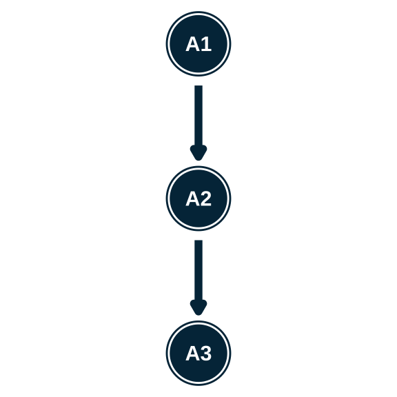
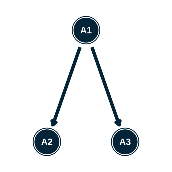
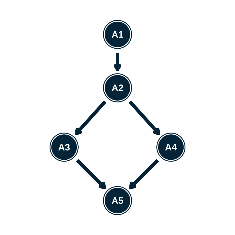
Exercise 2
- Write the hierarchy syntax for each of these structures
Estimating an attribute hierarchy
Exercise 3
We hypothesize that our PIE attributes follow a linear hierarchy
-
Fit an HDCM to the PIE data where Level 1 is required before Level 2, and Level 2 is required before Level 3
- Use MCMC as the method
- Use
"rstan"as the backend - Use 2 chains, each with 2000 total iterations, and 1000 warmup iterations
Testing our hypothesized structure
We can enforce a hierarchy on our model
Is that structure supported by the data we gathered?
-
Just like with the measurement models, we can use model comparisons to test our hypothesis
- Fit a model with all possible profiles
- Fit a model with only hypothesized profiles
If structure holds, the two models should be about equal (i.e., removing profiles doesn’t hurt anything)
Evaluating attribute structures with LOO
ecpe_spec <- dcm_specify(
  qmatrix = ecpe_qmatrix,
  identifier = "item_id",
  measurement_model = lcdm(),
  structural_model = unconstrained()
)

ecpe_lcdm <- dcm_estimate(
  dcm_spec = ecpe_spec,
  data = ecpe_data,
  identifier = "resp_id",
  method = "pathfinder",
  backend = "cmdstanr",
  single_path_draws = 1000,
  num_paths = 10,
  draws = 2000,
  file = here("materials", "slides", "fits", "ecpe-lcdm-uncst")
)Exercise 4
Compare our unconstrained model to the HDCM we just estimated
Which model is preferred? What does that tell us about our theory?
pie_lcdm_spec <- dcm_specify(
  qmatrix = pie_ft_qmatrix,
  identifier = "task",
  measurement_model = lcdm(),
  structural_model = unconstrained()
)

pie_lcdm <- dcm_estimate(
  pie_lcdm_spec,
  data = pie_ft_data,
  identifier = "student",
  method = "mcmc",
  backend = "rstan",
  chains = 2,
  iter = 2000,
  warmup = 1000,
  cores = 2,
  file = here("materials", "slides", "fits", "pie-lcdm-uncst")
)Structural models
Specification and estimation